Memory management is the heart of operating systems; it is crucial
for both programming and system administration. In the next few posts
I’ll cover memory with an eye towards practical aspects, but without
shying away from internals. While the concepts are generic, examples are
mostly from Linux and Windows on 32-bit x86. This first post describes
how programs are laid out in memory.
Each process in a multi-tasking OS runs in its own memory sandbox. This sandbox is the virtual address space, which in 32-bit mode is always a 4GB block of memory addresses. These virtual addresses are mapped to physical memory by page tables, which are maintained by the operating system kernel and consulted by the processor. Each process has its own set of page tables, but there is a catch. Once virtual addresses are enabled, they apply to all software running in the machine, including the kernel itself. Thus a portion of the virtual address space must be reserved to the kernel:
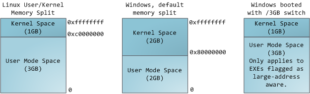 This does not mean the kernel uses that much
physical memory, only that it has that portion of address space
available to map whatever physical memory it wishes. Kernel space is
flagged in the page tables as exclusive to privileged code
(ring 2 or lower), hence a page fault is triggered if user-mode
programs try to touch it. In Linux, kernel space is constantly present
and maps the same physical memory in all processes. Kernel code and data
are always addressable, ready to handle interrupts or system calls at
any time. By contrast, the mapping for the user-mode portion of the
address space changes whenever a process switch happens:
This does not mean the kernel uses that much
physical memory, only that it has that portion of address space
available to map whatever physical memory it wishes. Kernel space is
flagged in the page tables as exclusive to privileged code
(ring 2 or lower), hence a page fault is triggered if user-mode
programs try to touch it. In Linux, kernel space is constantly present
and maps the same physical memory in all processes. Kernel code and data
are always addressable, ready to handle interrupts or system calls at
any time. By contrast, the mapping for the user-mode portion of the
address space changes whenever a process switch happens:
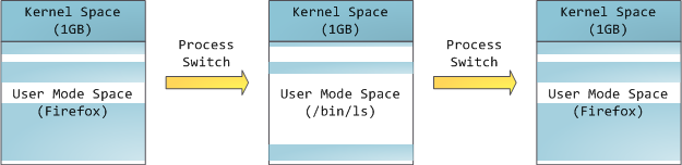 Blue regions represent virtual addresses that are mapped to physical
memory, whereas white regions are unmapped. In the example above,
Firefox has used far more of its virtual address space due to its
legendary memory hunger. The distinct bands in the address space
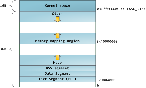
correspond to memory segments like the heap, stack, and so on. Keep in mind these segments are simply a range of memory addresses and have nothing to do with Intel-style segments. Anyway, here is the standard segment layout in a Linux process:
Blue regions represent virtual addresses that are mapped to physical
memory, whereas white regions are unmapped. In the example above,
Firefox has used far more of its virtual address space due to its
legendary memory hunger. The distinct bands in the address space
correspond to memory segments like the heap, stack, and so on. Keep in mind these segments are simply a range of memory addresses and have nothing to do with Intel-style segments. Anyway, here is the standard segment layout in a Linux process:
 When computing was happy and safe and cuddly, the starting virtual addresses for the segments shown above were exactly the same
for nearly every process in a machine. This made it easy to exploit
security vulnerabilities remotely. An exploit often needs to reference
absolute memory locations: an address on the stack, the address for a
library function, etc. Remote attackers must choose this location
blindly, counting on the fact that address spaces are all the same. When
they are, people get pwned. Thus address space randomization has become
popular. Linux randomizes the stack, memory mapping segment, and heap
by adding offsets to their starting addresses. Unfortunately the 32-bit
address space is pretty tight, leaving little room for randomization
and hampering its effectiveness.
When computing was happy and safe and cuddly, the starting virtual addresses for the segments shown above were exactly the same
for nearly every process in a machine. This made it easy to exploit
security vulnerabilities remotely. An exploit often needs to reference
absolute memory locations: an address on the stack, the address for a
library function, etc. Remote attackers must choose this location
blindly, counting on the fact that address spaces are all the same. When
they are, people get pwned. Thus address space randomization has become
popular. Linux randomizes the stack, memory mapping segment, and heap
by adding offsets to their starting addresses. Unfortunately the 32-bit
address space is pretty tight, leaving little room for randomization
and hampering its effectiveness.
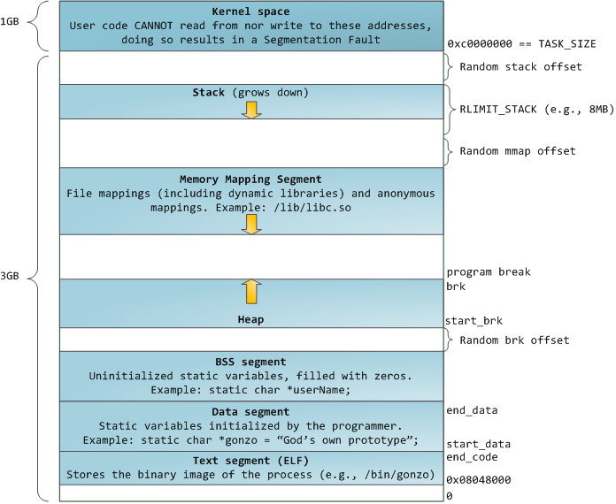
The topmost segment in the process address space is the stack, which stores local variables and function parameters in most programming languages. Calling a method or function pushes a new stack frame onto the stack. The stack frame is destroyed when the function returns. This simple design, possible because the data obeys strict LIFO order, means that no complex data structure is needed to track stack contents – a simple pointer to the top of the stack will do. Pushing and popping are thus very fast and deterministic. Also, the constant reuse of stack regions tends to keep active stack memory in the cpu caches, speeding up access. Each thread in a process gets its own stack.
It is possible to exhaust the area mapping the stack by pushing more data than it can fit. This triggers a page fault that is handled in Linux by expand_stack(), which in turn calls acct_stack_growth() to check whether it’s appropriate to grow the stack. If the stack size is below RLIMIT_STACK (usually 8MB), then normally the stack grows and the program continues merrily, unaware of what just happened. This is the normal mechanism whereby stack size adjusts to demand. However, if the maximum stack size has been reached, we have a stack overflow and the program receives a Segmentation Fault. While the mapped stack area expands to meet demand, it does not shrink back when the stack gets smaller. Like the federal budget, it only expands.
Dynamic stack growth is the only situation in which access to an unmapped memory region, shown in white above, might be valid. Any other access to unmapped memory triggers a page fault that results in a Segmentation Fault. Some mapped areas are read-only, hence write attempts to these areas also lead to segfaults.
Below the stack, we have the memory mapping segment. Here the kernel maps contents of files directly to memory. Any application can ask for such a mapping via the Linux mmap() system call (implementation) or CreateFileMapping() / MapViewOfFile() in Windows. Memory mapping is a convenient and high-performance way to do file I/O, so it is used for loading dynamic libraries. It is also possible to create an anonymous memory mapping that does not correspond to any files, being used instead for program data. In Linux, if you request a large block of memory via malloc(), the C library will create such an anonymous mapping instead of using heap memory. ‘Large’ means larger than MMAP_THRESHOLD bytes, 128 kB by default and adjustable via mallopt().
Speaking of the heap, it comes next in our plunge into address space. The heap provides runtime memory allocation, like the stack, meant for data that must outlive the function doing the allocation, unlike the stack. Most languages provide heap management to programs. Satisfying memory requests is thus a joint affair between the language runtime and the kernel. In C, the interface to heap allocation is malloc() and friends, whereas in a garbage-collected language like C# the interface is the new keyword.
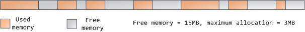
If there is enough space in the heap to satisfy a memory request, it can be handled by the language runtime without kernel involvement. Otherwise the heap is enlarged via the brk() system call (implementation) to make room for the requested block. Heap management is complex, requiring sophisticated algorithms that strive for speed and efficient memory usage in the face of our programs’ chaotic allocation patterns. The time needed to service a heap request can vary substantially. Real-time systems have special-purpose allocators to deal with this problem. Heaps also become fragmented, shown below:
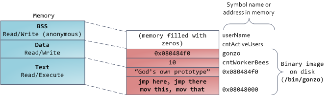
 Finally, we get to the lowest segments of memory: BSS, data, and
program text. Both BSS and data store contents for static (global)
variables in C. The difference is that BSS stores the contents of uninitialized
static variables, whose values are not set by the programmer in source
code. The BSS memory area is anonymous: it does not map any file. If you
say static int cntActiveUsers, the contents of cntActiveUsers live in the BSS.
Finally, we get to the lowest segments of memory: BSS, data, and
program text. Both BSS and data store contents for static (global)
variables in C. The difference is that BSS stores the contents of uninitialized
static variables, whose values are not set by the programmer in source
code. The BSS memory area is anonymous: it does not map any file. If you
say static int cntActiveUsers, the contents of cntActiveUsers live in the BSS.
The data segment, on the other hand, holds the contents for static variables initialized in source code. This memory area is not anonymous. It maps the part of the program’s binary image that contains the initial static values given in source code. So if you say static int cntWorkerBees = 10, the contents of cntWorkerBees live in the data segment and start out as 10. Even though the data segment maps a file, it is a private memory mapping, which means that updates to memory are not reflected in the underlying file. This must be the case, otherwise assignments to global variables would change your on-disk binary image. Inconceivable!
The data example in the diagram is trickier because it uses a pointer. In that case, the contents of pointer gonzo – a 4-byte memory address – live in the data segment. The actual string it points to does not, however. The string lives in the text segment, which is read-only and stores all of your code in addition to tidbits like string literals. The text segment also maps your binary file in memory, but writes to this area earn your program a Segmentation Fault. This helps prevent pointer bugs, though not as effectively as avoiding C in the first place. Here’s a diagram showing these segments and our example variables:
 You can examine the memory areas in a Linux process by reading the file /proc/pid_of_process/maps.
Keep in mind that a segment may contain many areas. For example, each
memory mapped file normally has its own area in the mmap segment, and
dynamic libraries have extra areas similar to BSS and data. The next
post will clarify what ‘area’ really means. Also, sometimes people say
“data segment” meaning all of data + bss + heap.
You can examine the memory areas in a Linux process by reading the file /proc/pid_of_process/maps.
Keep in mind that a segment may contain many areas. For example, each
memory mapped file normally has its own area in the mmap segment, and
dynamic libraries have extra areas similar to BSS and data. The next
post will clarify what ‘area’ really means. Also, sometimes people say
“data segment” meaning all of data + bss + heap.
You can examine binary images using the nm and objdump commands to display symbols, their addresses, segments, and so on. Finally, the virtual address layout described above is the “flexible” layout in Linux, which has been the default for a few years. It assumes that we have a value for RLIMIT_STACK. When that’s not the case, Linux reverts back to the “classic” layout shown below:
 That’s it for virtual address space layout. The next post discusses
how the kernel keeps track of these memory areas. Coming up we’ll look
at memory mapping, how file reading and writing ties into all this and
what memory usage figures mean.
That’s it for virtual address space layout. The next post discusses
how the kernel keeps track of these memory areas. Coming up we’ll look
at memory mapping, how file reading and writing ties into all this and
what memory usage figures mean.
Each process in a multi-tasking OS runs in its own memory sandbox. This sandbox is the virtual address space, which in 32-bit mode is always a 4GB block of memory addresses. These virtual addresses are mapped to physical memory by page tables, which are maintained by the operating system kernel and consulted by the processor. Each process has its own set of page tables, but there is a catch. Once virtual addresses are enabled, they apply to all software running in the machine, including the kernel itself. Thus a portion of the virtual address space must be reserved to the kernel:
The topmost segment in the process address space is the stack, which stores local variables and function parameters in most programming languages. Calling a method or function pushes a new stack frame onto the stack. The stack frame is destroyed when the function returns. This simple design, possible because the data obeys strict LIFO order, means that no complex data structure is needed to track stack contents – a simple pointer to the top of the stack will do. Pushing and popping are thus very fast and deterministic. Also, the constant reuse of stack regions tends to keep active stack memory in the cpu caches, speeding up access. Each thread in a process gets its own stack.
It is possible to exhaust the area mapping the stack by pushing more data than it can fit. This triggers a page fault that is handled in Linux by expand_stack(), which in turn calls acct_stack_growth() to check whether it’s appropriate to grow the stack. If the stack size is below RLIMIT_STACK (usually 8MB), then normally the stack grows and the program continues merrily, unaware of what just happened. This is the normal mechanism whereby stack size adjusts to demand. However, if the maximum stack size has been reached, we have a stack overflow and the program receives a Segmentation Fault. While the mapped stack area expands to meet demand, it does not shrink back when the stack gets smaller. Like the federal budget, it only expands.
Dynamic stack growth is the only situation in which access to an unmapped memory region, shown in white above, might be valid. Any other access to unmapped memory triggers a page fault that results in a Segmentation Fault. Some mapped areas are read-only, hence write attempts to these areas also lead to segfaults.
Below the stack, we have the memory mapping segment. Here the kernel maps contents of files directly to memory. Any application can ask for such a mapping via the Linux mmap() system call (implementation) or CreateFileMapping() / MapViewOfFile() in Windows. Memory mapping is a convenient and high-performance way to do file I/O, so it is used for loading dynamic libraries. It is also possible to create an anonymous memory mapping that does not correspond to any files, being used instead for program data. In Linux, if you request a large block of memory via malloc(), the C library will create such an anonymous mapping instead of using heap memory. ‘Large’ means larger than MMAP_THRESHOLD bytes, 128 kB by default and adjustable via mallopt().
Speaking of the heap, it comes next in our plunge into address space. The heap provides runtime memory allocation, like the stack, meant for data that must outlive the function doing the allocation, unlike the stack. Most languages provide heap management to programs. Satisfying memory requests is thus a joint affair between the language runtime and the kernel. In C, the interface to heap allocation is malloc() and friends, whereas in a garbage-collected language like C# the interface is the new keyword.
If there is enough space in the heap to satisfy a memory request, it can be handled by the language runtime without kernel involvement. Otherwise the heap is enlarged via the brk() system call (implementation) to make room for the requested block. Heap management is complex, requiring sophisticated algorithms that strive for speed and efficient memory usage in the face of our programs’ chaotic allocation patterns. The time needed to service a heap request can vary substantially. Real-time systems have special-purpose allocators to deal with this problem. Heaps also become fragmented, shown below:
The data segment, on the other hand, holds the contents for static variables initialized in source code. This memory area is not anonymous. It maps the part of the program’s binary image that contains the initial static values given in source code. So if you say static int cntWorkerBees = 10, the contents of cntWorkerBees live in the data segment and start out as 10. Even though the data segment maps a file, it is a private memory mapping, which means that updates to memory are not reflected in the underlying file. This must be the case, otherwise assignments to global variables would change your on-disk binary image. Inconceivable!
The data example in the diagram is trickier because it uses a pointer. In that case, the contents of pointer gonzo – a 4-byte memory address – live in the data segment. The actual string it points to does not, however. The string lives in the text segment, which is read-only and stores all of your code in addition to tidbits like string literals. The text segment also maps your binary file in memory, but writes to this area earn your program a Segmentation Fault. This helps prevent pointer bugs, though not as effectively as avoiding C in the first place. Here’s a diagram showing these segments and our example variables:
You can examine binary images using the nm and objdump commands to display symbols, their addresses, segments, and so on. Finally, the virtual address layout described above is the “flexible” layout in Linux, which has been the default for a few years. It assumes that we have a value for RLIMIT_STACK. When that’s not the case, Linux reverts back to the “classic” layout shown below:


 .
. .
. .
.


 .
.


